Tutorial

The tutorial’s test data can be found in the data folder of the GitHub repository. These datasets are a subsampled version of the multi-omics data sourced from Jeon et al., 2020. The test data includes three omics-related files along with accessory files:

1. Metabolomics abundance data: data/test_data/test.bac.abundance.csv

2. Metabolomics m/z data: data/test_data/test.bac.metabolome.csv

3. Transcriptomic expression matrix: data/test_data/test.bac.rnaseq.rpkm.csv

The RetroRules database is up-to-date and ready to use. The formatDatabase.py script is necessary only if you need to format older or revised database versions.”

Step 1 Query the LOTUS database

python queryMassNPDB.py -add docs/ESI-MS-adducts.csv -ms Jeon_tomato/test_data/test.bac.metabolome.csv -db lotus -dbp demo.sqlite -dtn Jeon_dummy_falcarindiol -t Solanum -dn test.sqlite -tn test_metabolites -c 20 -p 20 -v True

Note

The adducts file is available in the github repository data/ESI-MS-adducts.csv

Output

The script tentatively assigns annotations to each mass feature by identifying adducts and matching structures from the database to the ppm-adjusted precursor ion mass.

The outcomes are saved in the test.sqlite database within the test_metabolites table. The test data contains a total of 363 mass features, which, after processing with the queryMassNPDB_mod.py script, produced 2386 rows. This indicates that multiple structures are associated with each mass feature.

Step 2 Correlation analysis

Note

Make sure to keep the same column names in the transcriptomics and metabolomics CSV files

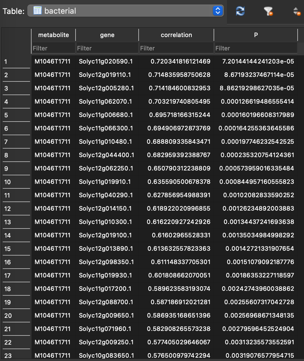
python corrMultiomics.py -ft data/test_data/test.bac.abundance.csv -qm data/test_data/test.bac.rnaseq.rpkm.csv -mr -cl -mad -r -c 0.1 -w 0.01 -mdr 5 10 25 50 -t 4 -dn test.sqlite -tn bacterial

This step saves the results in the test.sqlite database across various tables. The initial table, named bacterial, stores the correlation between each mass feature and individual transcripts/genes. Each correlation coefficient is accompanied by a p-value, indicating its statistical significance.

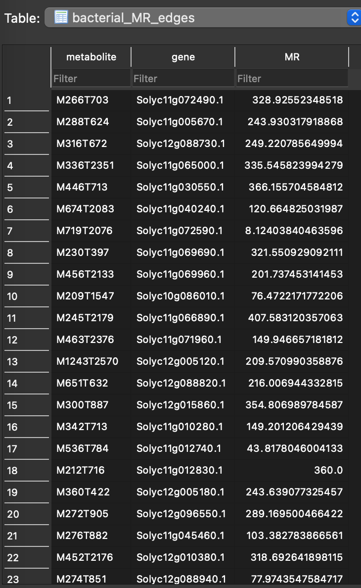
Correlation script converts correlation value into mutual ranks (MR). This information is stored in the database as bacterial_MR_edges table.

These MR values are processed through a decay function that transforms mutual ranks into edge scores. This transformation is crucial because the MR value can be as large as the number of features minus one (n-1, where n is the total number of features). To construct a network, a number between 0 and 1, derived from the MR, is required for use as edge weights. By default, MEANtools generates four networks using four different decay rates (5, 10, 25, & 50). The results are stored in four tables corresponding to these rates, named: bacterial_MR_edges_DR_5, bacterial_MR_edges_DR_10, bacterial_MR_edges_DR_25, and bacterial_MR_edges_DR_50.

To identify functional clusters (FCs; also known as modules or network hubs) within each corresponding network, MEANtools employs ClusterONE, a tool that utilizes edge weights to group genes and metabolites exhibiting similar expression and abundance patterns. The outcomes from ClusterONE are stored in four tables named: bacterial_clone_DR_5, bacterial_clone_DR_10, bacterial_clone_DR_25, and bacterial_clone_DR_50.

In this table, each row corresponds to a functional cluster. Various columns detail the characteristics of the FC, including its id, size (the count of genes and metabolites within the FC), density, the number of internal edges, the number of external edges, quality, and a p-value (which is calculated based on the inflow and outflow of edges from the FC). The final column enumerates the genes and metabolites, separated by spaces.

Note

Users can use this file to create networks using the plot_graph.py script.

Step 3 Merge Functional Clusters

After completing the correlation step, proceed to analyze the functional clusters derived from each network using different decay rates. This script facilitates the annotation of functional clusters and enables investigation into whether genes and metabolites from known pathways cluster together. Additional scripts provided in the GitHub repository can be used to generate network graphs based on these functional clusters.

python merge_clusters.py -ft data/test_data/test.bac.abundance.csv -qm data/test_data/test.bac.rnaseq.rpkm.csv -a -f data/test_data/pfams_description.csv -mc -mm overlap -dr 25 -dn test.sqlite

Based on the selected method for merging functional clusters, the script will combine FCs that share a common metabolite. The results of this merging process will be stored in the test.sqlite database under the table named merge_cluster_overlap_metabolite_DR_25. This table name reflects the merging method used (overlapping), the feature that prompted the merge (metabolite), and the network type (DR=25). The table consists of an identifier and merged genes and metabolites. This would be the final list of genes and metabolites that you want to take further to the prediction step.

Step 4 Map mass transitions

This step combines metabolome and transcriptome data with information from RR and MetaNetX. Essentially, it filters mass transitions linked to RR reactions based on the mass signatures present in the metabolome. For example, if there are no metabolites with a mass of 1000 in the metabolome, then the script will exclude reactions that involve masses of 1000.

python pathMassTransitions.py -c test_merged_cluster_filtered.csv -t test_db/format_database/MassTransitions.csv -dn test.sqlite -tn transitions_test -ct bacterial -mt test_metabolites -p Combined_small_middle_big_datasets.csv -a data/test_data/pfams.csv -s strict -cc 0.1 -cpc 1 -v

This step saves the results in the test.sqlite database within transitions_test. The script categorizes each meass feature as substrate and product and maps mass transitions estimated from the format database step.

Step 5 Predict reaction steps

This script integrates all data to produce pathway predictions. Here, all input is integreated, and all results are output as CSV tables that can be examined in a text editor, EXCEL, cytoscape.

python heraldPathways.py -c test_merged_cluster_filtered.csv -r test_db/format_database/ValidateRulesWithOrigins.csv -m test_db/format_database/base_rules.csv -p Combined_small_middle_big_datasets.csv -a data/test_data/bacterial.tomato.pfams.sol.csv -s loose -i 3 -dn test.sqlite -tn test_herald -ct bacterial -mt test_metabolites -tt transitions_test_falca -v -dv -o test_herald -d data/pfams_dict.csv

1. The first output file is a summary (Summary.csv) of the number of structures predicted in multiple iterations. Here initial structure is the number of stricture in the database. New structures are predicted in the virtual molecule generation process.

1. The second and third file output structures predicted along with their SMILES.

1. The third file constitutes the main results of the prediction. It is a CSV that list all mass features, mass transitions, structure annottaion, predicted reaction, SMILES, SMARTS, PFAM description, enzymes annotation, and correlations.

Named columns ms_substrate     ms_product      expected_mass_transition        predicted_mass_transition       mass_transition_difference      reaction_id     substrate_id    product_id      substrate_mnx   product_mnx     root    predicted_substrate_id  predicted_product_id    predicted_substrate_smiles      predicted_product_smiles        smarts_id       diameter        RR_substrate_smarts     RR_product_smarts       uniprot_id      uniprot_enzyme_pfams    KO      rhea_id_reaction        kegg_id_reaction        rhea_confirmation       kegg_confirmation       KO_prediction   gene    enzyme_pfams    correlation_substrate   P_substrate     correlation_product     P_product

Step 6 Generate reaction graphics

This step refines the results by producing visualizations and curated tables of predicted pathways, making them simpler to interpret. It generates tables and visualizations from the predicted reactions, filtering based on user specifications. The essential input for this script is the structure predictions from heraldPathways.

python paveWays.py -sp test_herald/structure_predictions.csv -of test_paveWays -r test_herald/reactions.csv -praf Combined_small_middle_big_datasets.csv -gaf data/test_data/pfams.csv -rr strict -pdg -pam -pup -v

The resulting folder structure looks like this:

The root structures are coming from the reactions file. Within root structures are the reaction steps (in SVG format) and CSV files that detail the reaction structures and scores (enzyme weight, edge weight and reaction score) asociated with each reaction step.

Generate reaction graphics with reaction likelihood scores

MEANtools generates reaction-likelihood scores based on substrate-enzyme association, for each anticipated reaction. To obtain the score, the likelihood of each atom in the substrate is calculated for being a site-of-metabolism using the GNN-SOM method. This results in an array of likelihoods for each atom in the substrate. Later, using ReactionDecoder, reaction centers and bond cleavages are predicted between each substrate and product. MEANtools makes use of this information to extract likelihood scores only for atoms that are involved in reaction centers and bond cleavages. The maximum value of likelihood score within the reaction center represents the reaction likelihood score.

To estimate reaction-likelihood scores for each predicted reactions, use the parameter –reaction_likelihood_scores or -rls

python paveWays.py -sp test_herald/structure_predictions.csv -of test_paveWays -r test_herald/reactions.csv -praf Combined_small_middle_big_datasets.csv -gaf data/test_data/pfams.csv -rr strict -pdg -pam -pup -v -rls -v -em EC-Pfam_calculated_associations_Extended.csv -rt

The reaction likelihood scores will be added in the structure_network.csv file inside the root_networks folder.